“有机会还是多学学, import tensorflow as torch!
前言
工作了一段时间,发现,外企工作氛围是真的好,具体感觉就是像又读了大学,什么都不会,什么都可以学,不打卡,超级人性化,哈哈哈 !
但是,我还是觉得有时间还是要好好学点东西,比如学点AI 知识,比如学学 import TensorFlow as torch ,这个帖子内容主要是 Udacity 的课,英文为主,我运行了一遍 jupyter notebook, 再搬到自己博客上面来,做碎片时间的复习吧,主要自用,记录自己的东西,有机会也会整理一点能看懂的中文笔记,比如怎么理解“drop out” 和“健身周一练胸,周二练背,周三练腿”的关系。不会的有好多,比如什么GAN , Bert , LSTM 都不知道…… 但是我确实都想学,最好有机会能做点东西出来,加油,实践确实是最好的学习方式! 那以后争取每周至少一篇吧。

正文
realize a Neural networks with PyTorch
Deep learning networks tend to be massive with dozens or hundreds of layers, that’s where the term “deep” comes from. You can build one of these deep networks using only weight matrices as we did in the previous notebook, but in general it’s very cumbersome and difficult to implement. PyTorch has a nice module nn that provides a nice way to efficiently build large neural networks.
# import some necessary  packages
import numpy as np
import torch

import helper

import matplotlib.pyplot as plt
and we will going to build a larger network that can slove the classic classfy problem “minist”. Here we’ll use the MNIST dataset which consists of greyscale handwritten digits. Each image is 28x28 pixels, you can see a sample below.
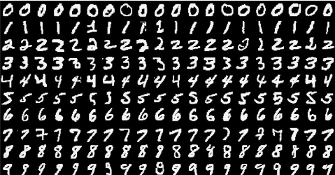
Our goal is to build a neural network that can take one of these images and predict the digit in the image.
First up, we need to get our dataset. This is provided through the torchvision package. The code below will download the MNIST dataset, then create training and test datasets for us. Don’t worry too much about the details here, you’ll learn more about this later.
from torchvision import datasets, transforms

# Define a transform to normalize the data
transform = transforms.Compose([transforms.ToTensor(),
                              transforms.Normalize((0.5,), (0.5,)),
                              ])

# Download and load the training data
trainset = datasets.MNIST('~/.pytorch/MNIST_data/', download=True, train=True, transform=transform)
trainloader = torch.utils.data.DataLoader(trainset, batch_size=64, shuffle=True)
We have the training data loaded into trainloader and we make that an iterator with iter(trainloader). Later, we’ll use this to loop through the dataset for training, like
for image, label in trainloader:
    ## do things with images and labels
You’ll notice I created the trainloader with a batch size of 64, and shuffle=True. The batch size is the number of images we get in one iteration from the data loader and pass through our network, often called a batch. And shuffle=True tells it to shuffle the dataset every time we start going through the data loader again. But here I’m just grabbing the first batch so we can check out the data. We can see below that images is just a tensor with size (64, 1, 28, 28). So, 64 images per batch, 1 color channel, and 28x28 images.
dataiter = iter(trainloader)
images, labels = dataiter.next()
print(type(images))
print(images.shape)
print(labels.shape)

## output
#<class 'torch.Tensor'>
#torch.Size([64, 1, 28, 28])
#torch.Size([64])
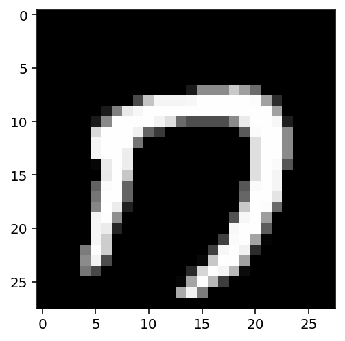
this is what one of the images looks like.
plt.imshow(images[1].numpy().squeeze(), cmap='Greys_r');
First, let’s try to build a simple network for this dataset using weight matrices and matrix multiplications. Then, we’ll see how to do it using PyTorch’s nn module which provides a much more convenient and powerful method for defining network architectures.
The networks you’ve seen so far are called fully-connected or dense networks. Each unit in one layer is connected to each unit in the next layer. In fully-connected networks, the input to each layer must be a one-dimensional vector (which can be stacked into a 2D tensor as a batch of multiple examples). However, our images are 28x28 2D tensors, so we need to convert them into 1D vectors. Thinking about sizes, we need to convert the batch of images with shape (64, 1, 28, 28) to a have a shape of (64, 784), 784 is 28 times 28. This is typically called flattening, we flattened the 2D images into 1D vectors.
Previously you built a network with one output unit. Here we need 10 output units, one for each digit. We want our network to predict the digit shown in an image, so what we’ll do is calculate probabilities that the image is of any one digit or class. This ends up being a discrete probability distribution over the classes (digits) that tells us the most likely class for the image. That means we need 10 output units for the 10 classes (digits). We’ll see how to convert the network output into a probability distribution next.
def activation(x):
    return 1/(1+torch.exp(-x))

# Flatten the input images
inputs = images.view(images.shape[0], -1)

# Create parameters
w1 = torch.randn(784, 256)
b1 = torch.randn(256)

w2 = torch.randn(256, 10)
b2 = torch.randn(10)

h = activation(torch.mm(inputs, w1) + b1)

out = torch.mm(h, w2) + b2
Now we have 10 outputs for our network. We want to pass in an image to our network and get out a probability distribution over the classes that tells us the likely class(es) the image belongs to. Something that looks like this:
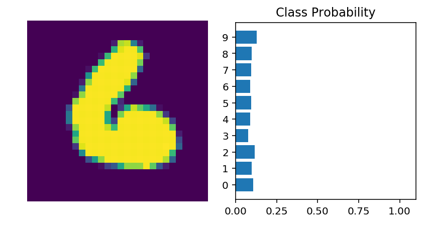
Here we see that the probability for each class is roughly the same. This is representing an untrained network, it hasn’t seen any data yet so it just returns a uniform distribution with equal probabilities for each class. To calculate this probability distribution, we often use the softmax function. Mathematically this looks like

What this does is squish each input 𝑥𝑖 between 0 and 1 and normalizes the values to give you a proper probability distribution where the probabilites sum up to one.
def softmax(x):
    ## TODO: Implement the softmax function here
     return torch.exp(x)/torch.sum(torch.exp(x), dim=1).view(-1, 1)

# Here, out should be the output of the network in the previous excercise with shape (64,10)
probabilities = softmax(out)

# Does it have the right shape? Should be (64, 10)
print(probabilities.shape)
# Does it sum to 1?
print(probabilities.sum(dim=1))
output:
torch.Size([64, 10])
tensor([1.0000, 1.0000, 1.0000, 1.0000, 1.0000, 1.0000, 1.0000, 1.0000, 1.0000,
        1.0000, 1.0000, 1.0000, 1.0000, 1.0000, 1.0000, 1.0000, 1.0000, 1.0000,
        1.0000, 1.0000, 1.0000, 1.0000, 1.0000, 1.0000, 1.0000, 1.0000, 1.0000,
        1.0000, 1.0000, 1.0000, 1.0000, 1.0000, 1.0000, 1.0000, 1.0000, 1.0000,
        1.0000, 1.0000, 1.0000, 1.0000, 1.0000, 1.0000, 1.0000, 1.0000, 1.0000,
        1.0000, 1.0000, 1.0000, 1.0000, 1.0000, 1.0000, 1.0000, 1.0000, 1.0000,
        1.0000, 1.0000, 1.0000, 1.0000, 1.0000, 1.0000, 1.0000, 1.0000, 1.0000,
        1.0000])
Building networks with PyTorch
PyTorch provides a module nn that makes building networks much simpler. Here I’ll show you how to build the same one as above with 784 inputs, 256 hidden units, 10 output units and a softmax output.
from torch import nn
class Network(nn.Module):
    def __init__(self):
        super().__init__()

        # Inputs to hidden layer linear transformation
        self.hidden = nn.Linear(784, 256)
        # Output layer, 10 units - one for each digit
        self.output = nn.Linear(256, 10)

        # Define sigmoid activation and softmax output
        self.sigmoid = nn.Sigmoid()
        self.softmax = nn.Softmax(dim=1)

    def forward(self, x):
        # Pass the input tensor through each of our operations
        x = self.hidden(x)
        x = self.sigmoid(x)
        x = self.output(x)
        x = self.softmax(x)

        return x
Let’s go through this bit by bit.
class Network(nn.Module):
Here we’re inheriting from nn.Module. Combined with super().__init__() this creates a class that tracks the architecture and provides a lot of useful methods and attributes. It is mandatory to inherit from nn.Module when you’re creating a class for your network. The name of the class itself can be anything.
self.hidden = nn.Linear(784, 256)
This line creates a module for a linear transformation, 𝑥𝐖+𝑏 , with 784 inputs and 256 outputs and assigns it to self.hidden. The module automatically creates the weight and bias tensors which we’ll use in the forward method. You can access the weight and bias tensors once the network (net) is created with net.hidden.weight and net.hidden.bias.
self.output = nn.Linear(256, 10)
Similarly, this creates another linear transformation with 256 inputs and 10 outputs.
    self.sigmoid = nn.Sigmoid()
    self.softmax = nn.Softmax(dim=1)
Here I defined operations for the sigmoid activation and softmax output. Setting dim=1 in nn.Softmax(dim=1) calculates softmax across the columns.
def forward(self, x):
PyTorch networks created with nn.Module must have a forward method defined. It takes in a tensor x and passes it through the operations you defined in the __init__ method.
x = self.hidden(x)
x = self.sigmoid(x)
x = self.output(x)
x = self.softmax(x)
Here the input tensor x is passed through each operation and reassigned to x. We can see that the input tensor goes through the hidden layer, then a sigmoid function, then the output layer, and finally the softmax function. It doesn’t matter what you name the variables here, as long as the inputs and outputs of the operations match the network architecture you want to build. The order in which you define things in the __init__ method doesn’t matter, but you’ll need to sequence the operations correctly in the forward method.
Now we can create a Network object.
# Create the network and look at it's text representation
model = Network()
model
output:
Network(
  (hidden): Linear(in_features=784, out_features=256, bias=True)
  (output): Linear(in_features=256, out_features=10, bias=True)
  (sigmoid): Sigmoid()
  (softmax): Softmax()
)
You can define the network somewhat more concisely and clearly using the torch.nn.functional module. This is the most common way you’ll see networks defined as many operations are simple element-wise functions. We normally import this module as F, import torch.nn.functional as F.
import torch.nn.functional as F

class Network(nn.Module):
    def __init__(self):
        super().__init__()
        # Inputs to hidden layer linear transformation
        self.hidden = nn.Linear(784, 256)
        # Output layer, 10 units - one for each digit
        self.output = nn.Linear(256, 10)

    def forward(self, x):
        # Hidden layer with sigmoid activation
        x = F.sigmoid(self.hidden(x))
        # Output layer with softmax activation
        x = F.softmax(self.output(x), dim=1)

        return x
Activation functions
So far we’ve only been looking at the sigmoid activation function, but in general any function can be used as an activation function. The only requirement is that for a network to approximate a non-linear function, the activation functions must be non-linear. Here are a few more examples of common activation functions: Tanh (hyperbolic tangent), and ReLU (rectified linear unit).
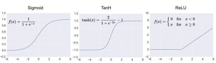
In practice, the ReLU function is used almost exclusively as the activation function for hidden layers.
Your Turn to Build a Network
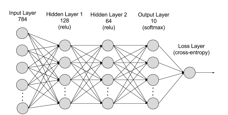
It’s good practice to name your layers by their type of network, for instance ‘fc’ to represent a fully-connected layer. As you code your solution, use fc1, fc2, and fc3 as your layer names.
## Your solution here
## Solution

class Network(nn.Module):
    def __init__(self):
        super().__init__()
        # Defining the layers, 128, 64, 10 units each
        self.fc1 = nn.Linear(784, 128)
        self.fc2 = nn.Linear(128, 64)
        # Output layer, 10 units - one for each digit
        self.fc3 = nn.Linear(64, 10)

    def forward(self, x):
        ''' Forward pass through the network, returns the output logits '''

        x = self.fc1(x)
        x = F.relu(x)
        x = self.fc2(x)
        x = F.relu(x)
        x = self.fc3(x)
        x = F.softmax(x, dim=1)

        return x

model = Network()
model
output:
Network(
  (fc1): Linear(in_features=784, out_features=128, bias=True)
  (fc2): Linear(in_features=128, out_features=64, bias=True)
  (fc3): Linear(in_features=64, out_features=10, bias=True)
)
Initializing weights and biases
The weights and such are automatically initialized for you, but it’s possible to customize how they are initialized. The weights and biases are tensors attached to the layer you defined, you can get them with model.fc1.weight for instance.
print(model.fc1.weight)
print(model.fc1.bias)

# output:
Parameter containing:
tensor([[-0.0330, -0.0197,  0.0181,  ..., -0.0280,  0.0169,  0.0311],
        [-0.0089,  0.0349,  0.0314,  ...,  0.0155, -0.0296,  0.0008],
        [-0.0151, -0.0280, -0.0109,  ..., -0.0349,  0.0264,  0.0317],
        ...,
        [-0.0128,  0.0089, -0.0020,  ...,  0.0089,  0.0082, -0.0281],
        [-0.0198,  0.0309, -0.0098,  ...,  0.0209, -0.0001, -0.0314],
        [ 0.0099,  0.0214,  0.0257,  ..., -0.0107, -0.0122,  0.0215]],
       requires_grad=True)
Parameter containing:
tensor([ 3.3122e-03, -2.2035e-03, -2.2405e-02,  6.6186e-03,  1.4285e-02,
        -2.0966e-03, -2.0341e-02,  3.4462e-02, -1.0969e-02, -2.2526e-02,
        -3.2171e-02,  2.0743e-02,  5.1247e-04,  1.2250e-03, -9.3866e-03,
        -3.0515e-03, -1.3425e-02,  2.6290e-02, -2.3399e-02, -2.7003e-02,
        -1.6268e-02, -3.2547e-02, -2.0991e-02,  1.5988e-02,  7.6564e-03,
         1.1219e-02, -2.0469e-02, -6.6756e-03,  1.5218e-02,  2.8958e-02,
         1.9062e-02, -1.3732e-02,  9.2672e-03, -1.9378e-02,  7.1341e-03,
        -3.3517e-02,  1.5284e-02,  2.0089e-02, -6.8955e-03, -2.5237e-02,
        -2.1829e-02, -1.9736e-02, -1.5000e-02, -2.4383e-02,  1.2065e-02,
        -3.4637e-02, -7.7769e-03,  1.3333e-02, -5.4149e-03, -3.3800e-02,
        -1.9812e-02,  1.1365e-02,  3.4652e-02,  1.9078e-02,  1.8352e-02,
        -2.0382e-03, -2.9273e-02,  3.0085e-02,  2.6071e-02,  2.2070e-02,
        -2.5921e-02, -3.1401e-02,  3.4565e-02, -3.1528e-02, -1.6730e-02,
        -1.8110e-03, -2.8110e-02, -5.2990e-03,  3.2715e-02, -1.5798e-02,
         2.6596e-02, -9.0170e-03,  5.8476e-04,  3.4375e-02,  3.0590e-02,
        -5.2098e-03,  3.4050e-02,  2.4159e-02, -2.2755e-02,  5.9574e-03,
        -3.3735e-02, -3.4779e-02,  1.6215e-02,  2.1917e-02, -3.3029e-02,
         2.3735e-02,  3.5215e-02,  8.7798e-05, -1.1952e-02,  3.7002e-03,
         2.5770e-02,  1.4461e-02, -3.4643e-02, -1.8159e-02, -5.9000e-03,
        -2.6111e-02,  2.7902e-03, -2.1747e-02,  3.0254e-03, -3.3776e-02,
         7.4499e-03, -8.0860e-03,  3.3299e-02,  3.3480e-02, -2.2713e-02,
        -3.0783e-02,  1.2280e-02,  9.6469e-03, -1.0758e-02, -1.4669e-02,
        -3.0705e-02,  3.2719e-02,  2.1025e-02,  2.3452e-02, -3.3599e-02,
        -7.0532e-03, -3.7518e-03, -1.1424e-03,  2.5243e-02, -3.0764e-02,
        -3.5027e-03, -3.0467e-02, -3.4664e-02,  1.1452e-02, -2.2981e-02,
         3.1746e-02,  3.4064e-03, -6.4315e-03], requires_grad=True)
For custom initialization, we want to modify these tensors in place. These are actually autograd Variables, so we need to get back the actual tensors with model.fc1.weight.data. Once we have the tensors, we can fill them with zeros (for biases) or random normal values.
# Set biases to all zeros
model.fc1.bias.data.fill_(0)

# ouput:
tensor([0., 0., 0., 0., 0., 0., 0., 0., 0., 0., 0., 0., 0., 0., 0., 0., 0., 0., 0., 0., 0., 0., 0., 0.,
        0., 0., 0., 0., 0., 0., 0., 0., 0., 0., 0., 0., 0., 0., 0., 0., 0., 0., 0., 0., 0., 0., 0., 0.,
        0., 0., 0., 0., 0., 0., 0., 0., 0., 0., 0., 0., 0., 0., 0., 0., 0., 0., 0., 0., 0., 0., 0., 0.,
        0., 0., 0., 0., 0., 0., 0., 0., 0., 0., 0., 0., 0., 0., 0., 0., 0., 0., 0., 0., 0., 0., 0., 0.,
        0., 0., 0., 0., 0., 0., 0., 0., 0., 0., 0., 0., 0., 0., 0., 0., 0., 0., 0., 0., 0., 0., 0., 0.,
        0., 0., 0., 0., 0., 0., 0., 0.])
# sample from random normal with standard dev = 0.01
model.fc1.weight.data.normal_(std=0.01)

# output:
tensor([[-0.0089,  0.0016,  0.0087,  ..., -0.0102, -0.0076, -0.0059],
        [ 0.0083, -0.0046, -0.0021,  ...,  0.0072, -0.0009, -0.0049],
        [-0.0128,  0.0022,  0.0047,  ...,  0.0031, -0.0119, -0.0051],
        ...,
        [-0.0008,  0.0190, -0.0062,  ..., -0.0141, -0.0018,  0.0024],
        [ 0.0047,  0.0122, -0.0016,  ..., -0.0061, -0.0031,  0.0082],
        [ 0.0166, -0.0056, -0.0128,  ...,  0.0011, -0.0101, -0.0141]])
Forward pass
Now that we have a network, let’s see what happens when we pass in an image.
# Grab some data
dataiter = iter(trainloader)
images, labels = dataiter.next()

# Resize images into a 1D vector, new shape is (batch size, color channels, image pixels)
images.resize_(64, 1, 784)
# or images.resize_(images.shape[0], 1, 784) to automatically get batch size

# Forward pass through the network
img_idx = 0
ps = model.forward(images[img_idx,:])

img = images[img_idx]
helper.view_classify(img.view(1, 28, 28), ps)
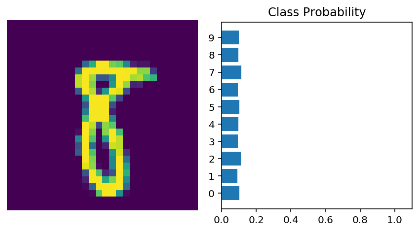
As you can see above, our network has basically no idea what this digit is. It’s because we haven’t trained it yet, all the weights are random!
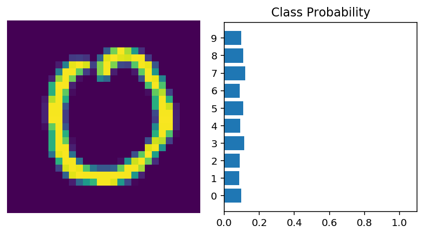
Using nn.Sequential PyTorch provides a convenient way to build networks like this where a tensor is passed sequentially through operations, nn.Sequential (documentation). Using this to build the equivalent network:
# Hyperparameters for our network
input_size = 784
hidden_sizes = [128, 64]
output_size = 10

# Build a feed-forward network
model = nn.Sequential(nn.Linear(input_size, hidden_sizes[0]),
                      nn.ReLU(),
                      nn.Linear(hidden_sizes[0], hidden_sizes[1]),
                      nn.ReLU(),
                      nn.Linear(hidden_sizes[1], output_size),
                      nn.Softmax(dim=1))
print(model)

# Forward pass through the network and display output
images, labels = next(iter(trainloader))
images.resize_(images.shape[0], 1, 784)
ps = model.forward(images[0,:])
helper.view_classify(images[0].view(1, 28, 28), ps)


# outputs
# Sequential(
  (0): Linear(in_features=784, out_features=128, bias=True)
  (1): ReLU()
  (2): Linear(in_features=128, out_features=64, bias=True)
  (3): ReLU()
  (4): Linear(in_features=64, out_features=10, bias=True)
  (5): Softmax()
)
Here our model is the same as before: 784 input units, a hidden layer with 128 units, ReLU activation, 64 unit hidden layer, another ReLU, then the output layer with 10 units, and the softmax output.
The operations are available by passing in the appropriate index. For example, if you want to get first Linear operation and look at the weights, you’d use model[0].
print(model[0])
model[0].weight

# outputs:

Linear(in_features=784, out_features=128, bias=True)
Parameter containing:
tensor([[-1.9726e-02, -2.6318e-02,  7.3969e-04,  ..., -2.7043e-02,
          2.5223e-02, -1.7928e-02],
        [-4.6518e-05,  3.8646e-04,  9.2211e-03,  ...,  3.3658e-02,
         -1.3175e-02,  1.0972e-02],
        [-1.5371e-02,  2.7720e-02,  3.4194e-02,  ..., -1.2030e-02,
         -4.1426e-03,  3.8336e-03],
        ...,
        [-2.3057e-02,  1.6326e-02, -2.4367e-02,  ..., -3.2292e-02,
         -1.1982e-02, -3.0219e-02],
        [ 3.2814e-03, -7.2229e-03,  3.3498e-02,  ..., -2.3360e-02,
          8.5508e-03,  3.3357e-03],
        [ 2.4090e-02,  2.7164e-02,  2.8544e-02,  ..., -2.3281e-02,
         -2.4122e-02,  9.2324e-03]], requires_grad=True)
You can also pass in an OrderedDict to name the individual layers and operations, instead of using incremental integers. Note that dictionary keys must be unique, so each operation must have a different name.
from collections import OrderedDict
model = nn.Sequential(OrderedDict([
                      ('fc1', nn.Linear(input_size, hidden_sizes[0])),
                      ('relu1', nn.ReLU()),
                      ('fc2', nn.Linear(hidden_sizes[0], hidden_sizes[1])),
                      ('relu2', nn.ReLU()),
                      ('output', nn.Linear(hidden_sizes[1], output_size)),
                      ('softmax', nn.Softmax(dim=1))]))
model

# outputs
Sequential(
  (fc1): Linear(in_features=784, out_features=128, bias=True)
  (relu1): ReLU()
  (fc2): Linear(in_features=128, out_features=64, bias=True)
  (relu2): ReLU()
  (output): Linear(in_features=64, out_features=10, bias=True)
  (softmax): Softmax()
)
Now you can access layers either by integer or the name
print(model[0])
print(model.fc1)

# outputs
Linear(in_features=784, out_features=128, bias=True)
Linear(in_features=784, out_features=128, bias=True)